Mapping
Maps are graphical representations of geolocalized information. In the context of robotics, mapping can be defined as the task of building maps using robotics platforms. Mapping is one of the most common tasks for mobile robots: mobile robots can freely move in their environment and record, process, and transmit information to a remote operator. The nature of the maps that a robot can build are determined by its set of sensors. For example, sensors that detect obstacles can be used to map the occupation of the environment, and sensors that detect gases can be used to map their concentration in different locations of the robot’s workspace.
As it might result evident, mapping implies that the robot is capable of determining where it is. This information can be provided externally by navigation systems such as GPS, or it can be computed internally by the robot. When it is computed internally, sensors like the encoders of the wheels, gyroscopes, inertial measurement units (IMU), and computer vision systems can provide information of the displacement of the robot. By integrating this information over the time, it is possible to estimate where the robot is—in the same way that your mobile phone integrate its sensory information to estimate your pose in systems like Google Maps.
If no sensor can provide information about the displacement of the robot, a similar result can be obtained by integrating the velocity commands that the robot receives. Obtaining an estimation of the pose of the robot out of the integration of its sequential movements is often referred so as odometry .
Objective
The objective of this practical session is to estimate the pose of the robot out of the velocity commands it receives, and after, to build a map of its workspace.
General remarks
In this and the following practical sessions, it will be understand that pose refers to the position and orientation of the robot.
This practical session has two exercises: first, you will compute a simplified version of the odometry of the robot; later, you will teleoperate the robot, build a map of its environment, and locate objects of interest in the map. In the first exercise you will write code in the corresponding python script. In the second exercise you will be asked only to drive the robot, and record and organize information.
You can enter the directory of this practical session by entering the commands
cd ~/catkin_ws/src/mapping/scripts
There you will find the file odometry_node.py—the script that you will use to compute the odometry of the robot.
IMPORTANT: 1 - Set the properties of the file for being executable.
chmod +x odometry_node.py
2 - Execute this extra command to patch the script to run in Ubuntu 20.04
sed -i 's/python/python3/g' odometry_node.py
3 - Add the following lines into the script odometry_node.py. They must be placed with the rest of pre-defined global variables.
# Pre-defined global variables

_model_index = 0       # New line to be added
_model_found = False   # New line to be added
_odometry = Pose2D()
_truth_pose = Pose2D()
_cmd_vel = Twist()
_last_time = rospy.Time(0)
By mistake, they are missing in the script that you downloaded.
4 - Then, download the extra models required for this practical session.
cd
wget --load-cookies /tmp/cookies.txt "https://docs.google.com/uc?export=download&confirm=$(wget --quiet --save-cookies /tmp/cookies.txt --keep-session-cookies --no-check-certificate 'https://docs.google.com/uc?export=download&id=1PXc8AOdUpTZZhInzSwopFyBNxNQvoci6' -O- | sed -rn 's/.*confirm=([0-9A-Za-z_]+).*/\1\n/p')&id=1PXc8AOdUpTZZhInzSwopFyBNxNQvoci6" -O preloaded_models.tar.xz && rm -rf /tmp/cookies.txt
You can know that the download process has finished when the terminal shows you an output similar to the one below.
2022-10-18 00:50:26 (597 KB/s) - ‘preloaded_models.tar.xz’ saved [54243716/54243716]
Once the download finishes, decompress the file using the command
tar -xvf preloaded_models.tar.xz --directory ~/.gazebo/models/.
Exercise 1: odometry
Odometry is the process of estimating the pose of a robot with respect to an arbitrary pose where the robot was at an arbitrary past time. The odometry estimates the current pose by incrementally integrating its movement at each control cycle.
In pseudocode, it could be defined as
newPose = oldPose + estimatedMovement
And a graphical representation is shown below
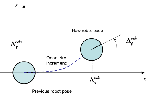
Hence, the first pose registered by the odometry will set the coordinate system on which subsequent estimations will be framed. For example, if the odometry starts at the beginning of the experiment, the odometry will be an estimation of the pose of the robot with respect to the pose of the robot at the beginning of the experiment.
The accuracy of the estimations in the odometry can be affected by non-systematic and systematic errors. Non-systematic errors often cannot be measured and can be caused by uneven friction of the surface, wheel slippage, bumps, among others. Systematic errors are caused due to differences of the model of the robot and its real functioning—for example, if the velocity we command always differ by a fixed value with the real one.
The accuracy of the odometry will be reduced over time due to the cumulative effect of non-systematic and systematic errors.
In the practical session P1.1 you sent velocity commands to drive the robot on its scenario. In this exercise, you will use those commands to estimate the pose of the robot using odometry—the pose will be estimated with respect to the pose of the robot when the experiment is launched.
Launching the experiment
1 - Open a terminal and enter the directory that contains the materials for this practical session.
cd ~/catkin_ws/src/mapping/scripts
2 - Run the simulation in Gazebo.
roslaunch mapping sandbox.launch
Experimental setup
At the beginning of the experiment, the Summit-XL is spawned in the scenario you explored in the practical session P1.0. The initial pose of the robot is at the coordinates (x,y,z) (0,0,0), with an orientation theta of 0.0°.
Computing the odometry
In this exercise you will use a simplified model of the robot to compute the odometry. In this simplified model, we assume that the movement of the robot can be described by linear displacements and rotations that happen one after the other—instead of describing arch trajectories. The movement of the robot is described by its linear velocity Vx and its angular velocity Wz, and the odometry can be estimated by summing at each time step the movement of the robot.
You can compute the odometry using the following pseudocode
1 - Estimate the time difference between the last and the current time step.
2 - Compute the position change in the x coordinate due to Vx
delta_x = (linear_velocity * cos(current_orientation)) * time_difference
3 - Compute the position change in the y coordinate due to Vx
delta_y = (linear_velocity * sin(current_orientation)) * time_difference
4 - Compute the orientation change in theta due to Wz
delta_theta = angular_velocity * time_difference
5 - Update the pose of the robot by summing the last and current pose.
6 - Normalize the orientation theta of the robot between [-pi,pi]
7 - Set the values in the odometry output
Testing the odometry
You can move the robot using the Linux terminal or the interface you developed in the practical session,P1.0. At any time, you can test your implementation by running the script with the command
rosrun mapping odometry_node.py
If no error is reported, you can try moving the robot. If you wish to try something else, click on the terminal running the teleoperation interface and press Ctrl + C until the process stops.
If you wish to check the output of your implementation, open a new terminal and enter the command
rostopic echo /robot/mapping/estimated_odometry
You can compare your implementation with the position provided by the odometry computed by the robot. At this moment is not possible to compare the orientation, however, the position should be enough to make comparisons. To do so, open a new terminal and enter the command
rostopic echo /robot/robotnik_base_control/odom/pose/pose/position
You can also compare your estimation, and the one of the robot, with the real pose provided by the simulator—imaging that you are comparing your solution with a GPS. You can get the real pose of the robot with the command
rostopic echo /robot/mapping/truth_pose
To be considered
Try first moving the robot with linear velocities. How good is your estimation in comparison to the one of the robot, and the real pose that you get from the simulator?
What do you observe when you start rotating the robot? What if you try arch trajectories?
Proposed solution
A proposed solution for the exercise will be available to download after midnight.
Exercise 2: mapping
Now you know how to get the pose of the robot in the scenario, both the one you estimated and the real one. In this exercise you will use the Summit XL to explore an unknown scenario, build a map, locate objects of interest, and provide useful information about the scenario.
In this exercise, you will use the interface you developed in the session P1.1 to drive the robot, and your implementation from the first exercise of this session to get the estimated position and the real position of the robot.
Launching the experiment
1 - Open a terminal and enter the directory that contains the materials for this practical session.
cd ~/catkin_ws/src/mapping/scripts
2 - Run the simulation in Gazebo.
roslaunch mapping mapping.launch
This time, the Gazebo interface will not be spawned. You will get a new interface named ´RViz´ in which you can visualize the readings of the sensors of the robot.
Experimental setup
At the beginning of the experiment, the Summit-XL is spawned in the football field, that now is cluttered with objects. The initial pose of the robot is at the coordinates (x,y,z) (0,0,0), with an orientation theta of 0.0°. The interface and its components are indicated below.
The RViz interface
RViz shows you two windows: the window in the left displays the readings of the camera, and the window in the right displays the map that the robot is building.
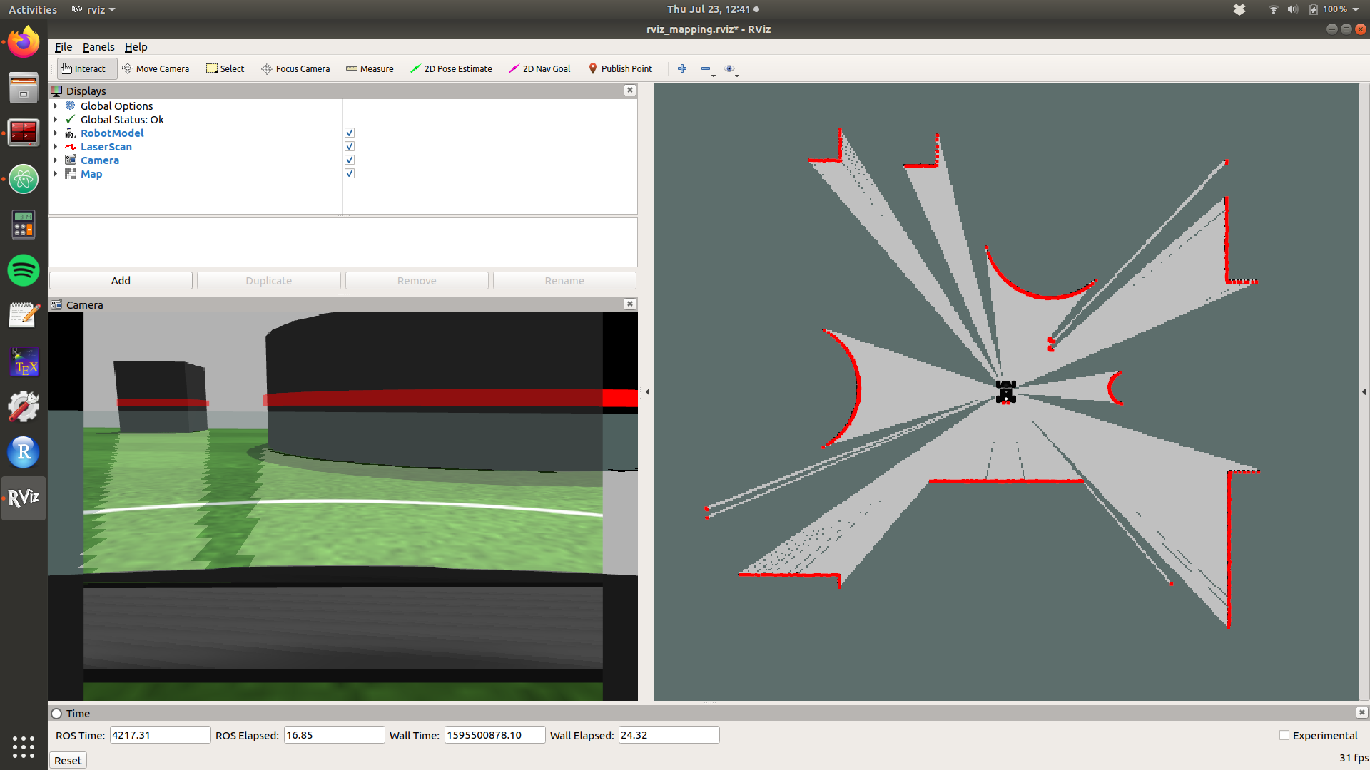
As mentioned in the user guide of the Summit-XL, the robot has a LIDAR that can be used to detect surrounding objects. The readings of this sensor are displayed in red in the camera window and in the map window.
You can also see projections of the map that is being built in the camera window. This projections can be seen as gray shades that overlap the floor of the football field.
Building the map
The Summit-XL has been already configured to build a map for you. The robot uses its 360° LIDAR to get information about surrounding obstacles in a distance of up to 10 m. While moving in the scenario, the robot compares its estimated position with position of the objects it perceives. This method is called simultaneous localization and mapping (SLAM). The robot estimates first its pose, and later, it incrementally builds a map by registering its estimated pose, and the one of the objects it perceives.
In this part of the exercise, you only need to drive the robot in the scenario. The readings of the LIDAR and pose of the robot are automatically registered and used to build the map you see in the right window.
Finding objects of interest and providing metrics
You will be given with 3 different types of objects of interest that you must find the scenario, and locate in the map. In this part of the exercise, when you see an object of interest, you must estimate and register manually the position of the object by using both your estimated odometry and the pose of the robot provided by the simulator—see Exercise 1. You will use later that information to position the objects in the map, and compare the map you obtain with your odometry and with the real position of the robot.
In total, you can find 4 people, 4 construction signs, and 7 ground robots. The objects are shown below.
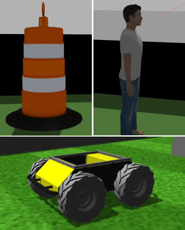
Finally, you must also estimate the dimensions of the football using the robot.
Saving the map
After you are done exploring, and you completely build the map, you can save the map. First, enter the directory of the exercise
cd ~/catkin_ws/src/mapping/scripts
After, you can save the map with the command
rosrun map_server map_saver map:=/robot/map
You will get a file named map.yaml that contains metadata of the map, and an image map.pgm.
The map will be saved in the directory in which you run the command. If a map already exists, it might overlap the one you had.
Delivering the map
As the purpose of building maps is to provide a graphical representation of the scenario, you deliver a map that indicates the dimensions of the football, and the position of the objects of interest you found.
Proposed solution
A proposed solution for the exercise will be available to download after midnight.
Further readings
The following reading discusses advances in simultaneous localization and mapping (SLAM).
1 - Khairuddin, A. R. et al. (2015). Review on simultaneous localization and mapping (SLAM).